Beam Search

Intelligently generating a linguistically coherent sequence of words is an important feature of a wide range of modern NLP applications like machine translation, chatbots, question answering, etc.. The process of sequence generation boils down to repeatedly performing a simple action: spitting out the next word based on the current word (and implicitly all the words that have been generated so far), which is implemented by a function or subroutine that computes a probability distribution over all legitimate next words and decides which word to output according to that prob distribution.

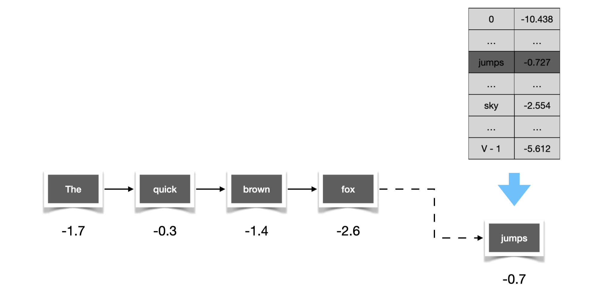
Figure 1. Generate sequence by repeatedly picking the next word.

Informally, we are interested in finding a sequence that is most likely to be generated, which is quantified by the probability score of the sequence, or equivalently the sum of logarithm of probabilities (sum-of-log-probs) of its constituent words. While it might be straightforward to let the function output whichever word with the largest probability throughout the entire process, it’s worth noting that the function has a unique property in that it takes in its own output at previous time steps to compute the current output, and as a result the prob distribution of next word may vary depending on the choice we made in the past. As we will see shortly, this property has subtle implication on our word-picking strategy — picking words with lower probabilities, a seemingly non-optimal move, may eventually pay off as it unlocks access to choices that may lead to overall higher score of the entire sequence.

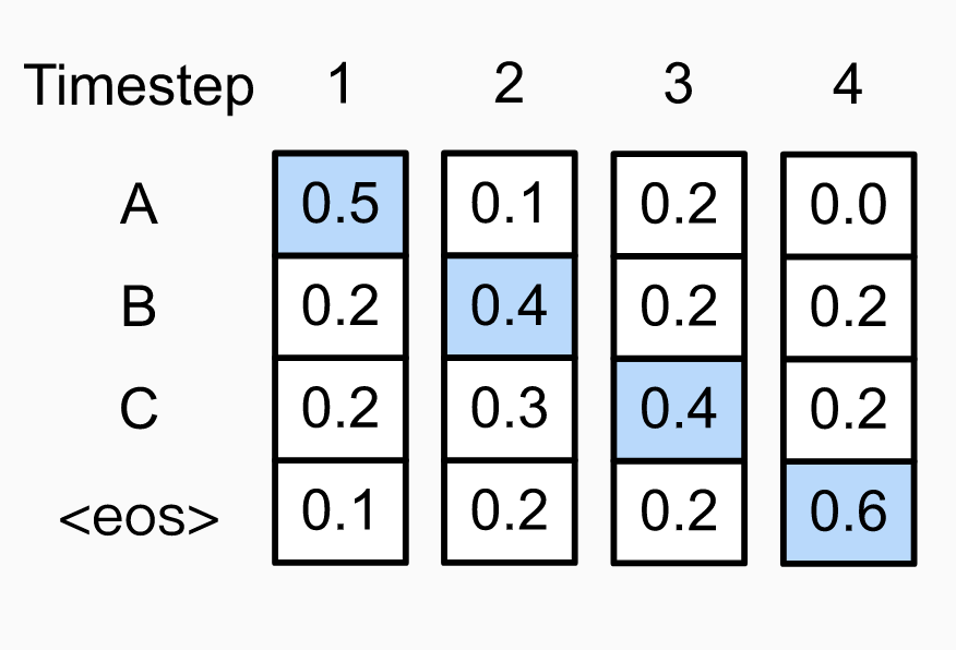
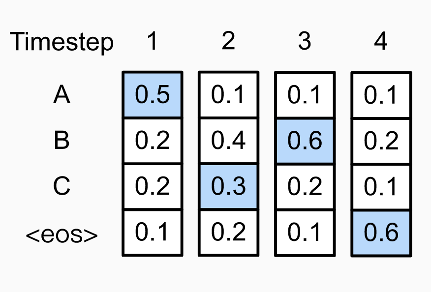
Figure 2. Left: sequence "ABC" found by greedy search with probability 0.048; Right: optimal sequence "ACB" with probability 0.054. Note the probability distribution diverges starting from time step 3, because different choices were made at the preceding step ("C" vs. "B"). The search leading to the globally optimal sequence made a locally non-optimal choice at time step 2. Image credit: [http://www.d2l.ai/chapter_recurrent-modern/beam-search.html]

Intuition

So what would be a good word-picking strategy? Notice that we are essentially facing a tree search problem – We start off with a single partial sequence that contains only the special word SOS (Start Of Sequence), together with its sum-of-log-probs (i.e. $0=\log 1$ ). We would like to consider each word from the vocabulary as a potential next word of the current partial sequence, so we duplicate it to $V$ (vocabulary size) copies and each copy gets extended with a different word. Then we update the sum-of-log-probs of the $V$ partial sequences that are now one word longer. Obviously we are going to end up with an exponential search space of $V^n$ sequences if we were to repeat this process for $n$ steps, which would make any algorithm that seeks to exhaustively search for the sequence with largest sum-of-log-probs computationally intractable.

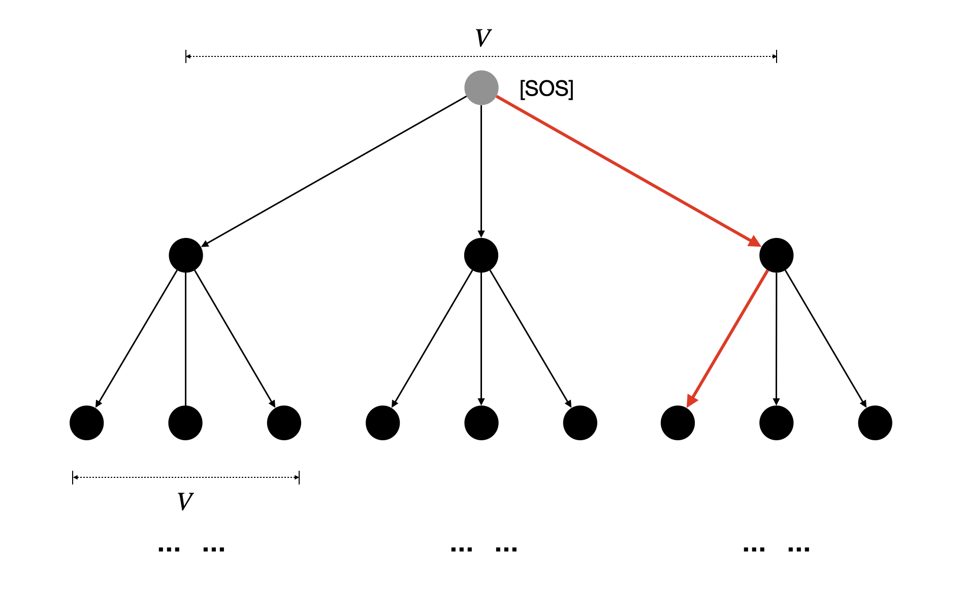
Figure 3. Exhaustive Search expands the search tree unboundedly. Each root-to-leaf path corresponds to a candidate sequence.

Rather than let the search space grow unboundedly with the length of sequence, Beam Search limits the total number of sequences that we are tracking to a constant $k$ (a.k.a. beam width). Like exhaustive search, when we expand the current set of $k$ candidate partial sequences (a.k.a. beams) of length $l$ , we consider each of the $V$ vocabulary words as the potential next word, leading to $kV$ sequences of length $l + 1$ . Unlike exhaustive search, we prune all but the top $k$ most promising (with largest sum-of-log-probs) candidates, bringing the “candidate pool” back to the original size. However, the downside is that there is no guarantee Beam Search is going to find the same optimal solution as the exhaustive search, because the goal state leading to optimality may have been pruned halfway. In this sense, Beam Search is a heuristic algorithm that sacrifices completeness for tractability.

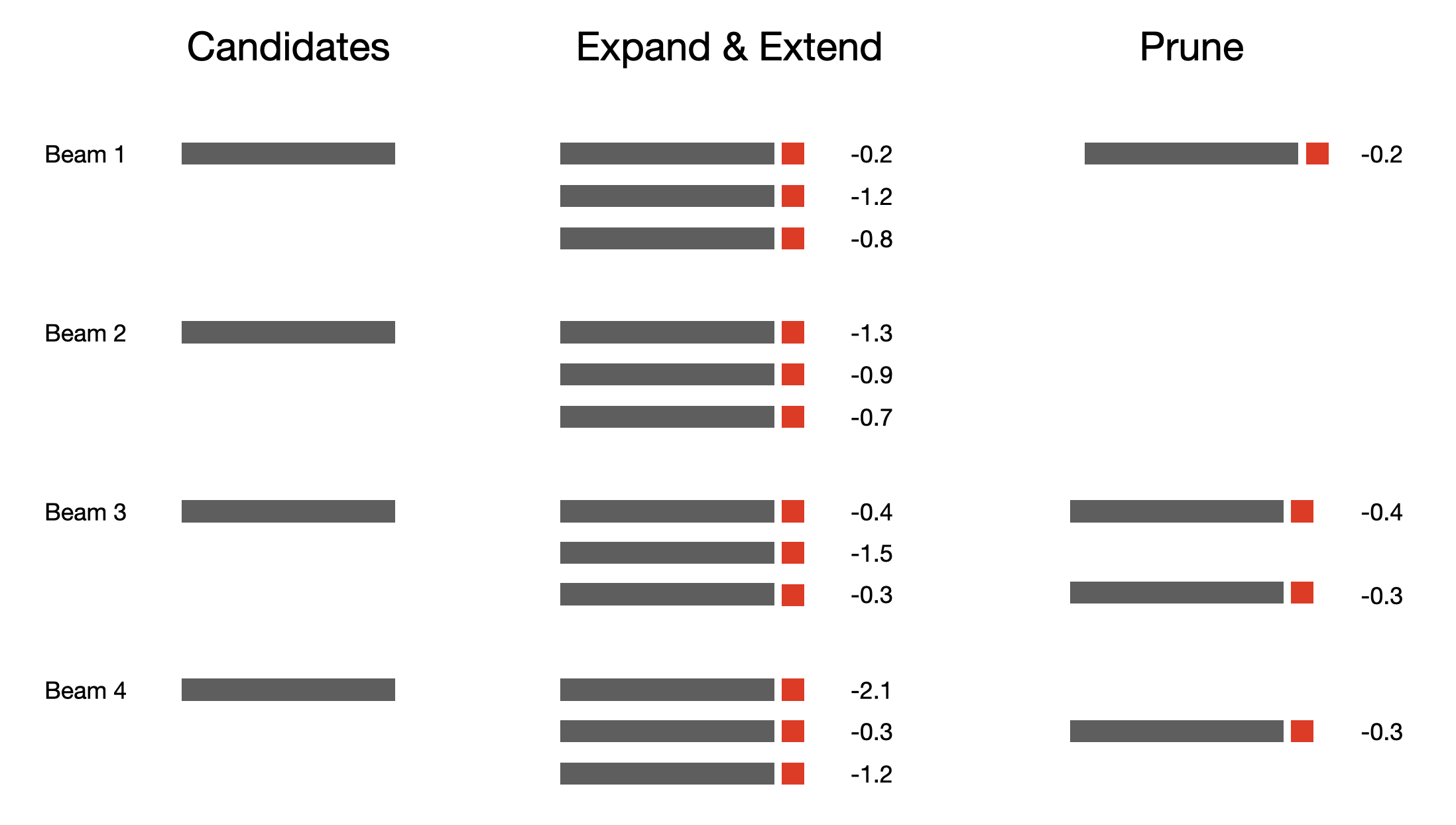
Figure 4. Beam Search prunes candidate sequences to a constant size k=4. Candidates first get extended by one word and expanded by a factor of V=3, then get pruned back to beam width k=4.

Implementation

Now that we have some intuition about how Beam Search works in general, let’s get to the nuts and bolts of the algorithm that we need to understand to implement it correctly.

Each beam maintains its own set of states

At this point you should already be convinced that we need to keep track of the status of each beam as we grow the partial sequences. We create ndarrays active_seqs and active_log_probs with shape [batch_size, beam_width, partial_seq_len] and [batch_size, beam_width], respectively, where the slices into the beam dimension, active_seqs[:, j] and active_log_probs[:, j], store the status of beam j, i.e. the list of word IDs making that partial sequence and the corresponding sum-of-log-prob.

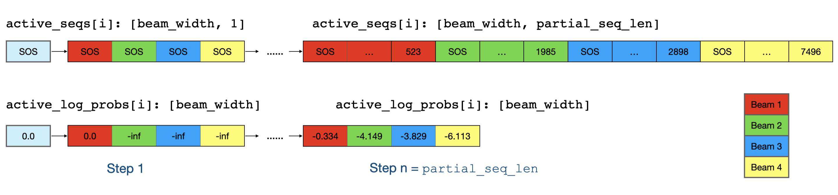
Figure 5. Initial setup of active partial sequences & their sum-of-log-probs, and what they look like a few steps into the searching process. For example, the sum-of-log-prob of the partial sequence [SOS, ..., 523] equals -0.334 aftern Step n.

As shown in Figure 5, we started with a single copy of the initial partial sequence (SOS) and its sum-of-log-prob (0.0), and we need to duplicate them to beam_width copies so each beam gets its own set of states. However, if we were to simply copy the initial value of sum-of-log-prob across all beams, we would end up with identical partial sequences after “Step 1”. The trick is to “suppress” the sum-of-log-probs of partial squences coming from all but the first beam, so only those sequences will “survive” after the pruning (See Figure 6).

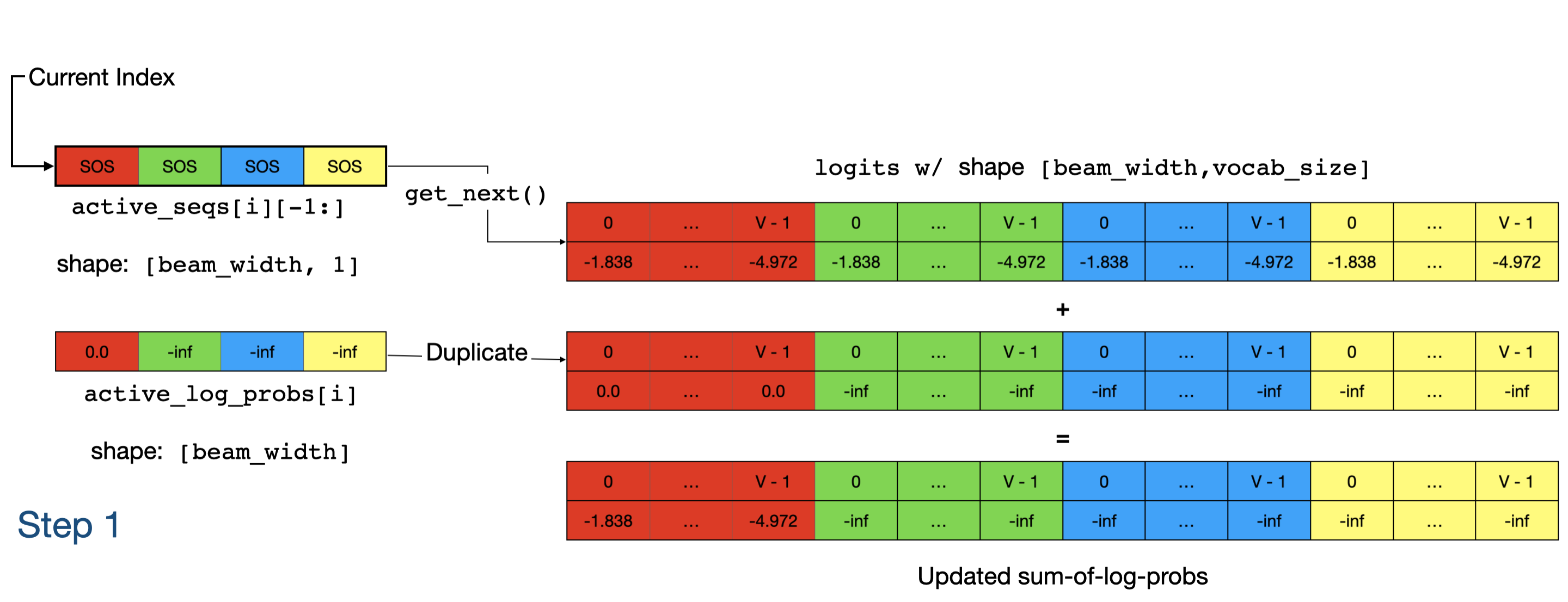
Figure 6. Computing logits of "next words" (by calling get_next()) and updating the sum-of-log-probs (by adding "logits" with duplicated "active_log_probs[i]"). Note that the distributions of the logits of "next words" are the same across different beams because the same input "SOS" was fed to get_next(); and the -inf entries in "active_log_probs[i]" push the scores of partial sequences from Beam 2, 3, and 4 to -inf, so we are effectively picking top scoring candidates only from Beam 1.

You may have noticed that some variable names we referenced are prefixed with active_. By that we mean they are still being actively extended, untill we stumble across EOS (like SOS), which is another special word from the vocabulary that signals the End of Sequence. We say those partial sequences ending with EOS are in the finished state (as opposed to active), and their states will be stored in ndarrays other than active_seqs and active_log_probs. Intuitively, active sequence plays the role of “frontiers” as we explore the search space, whereas finished sequence records those that are indeed “finished” and are ready to output. We want to make sure that the width of the frontier (i.e. number of active sequences) is unchanged throughout the course of Beam Search.

How states are updated

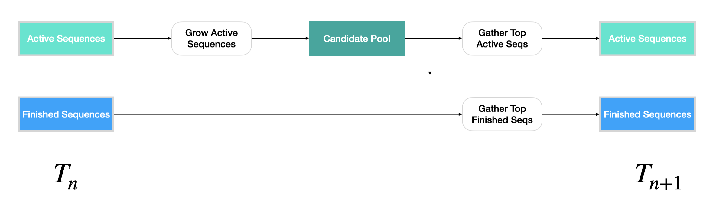
Figure 7. Overview of how active and finished sequences are updated within a single step of Beam Search.

Now we are ready to explain exactly what happens in a single step of Beam Search, where the partial sequences get extended by one word and their sum-of-log-probs get updated accordingly. The main logic can be broken down into three substeps:

Grow Active Sequences
Gather Top Active Sequences
Gather Top Finished Sequences

Grow Active Sequences

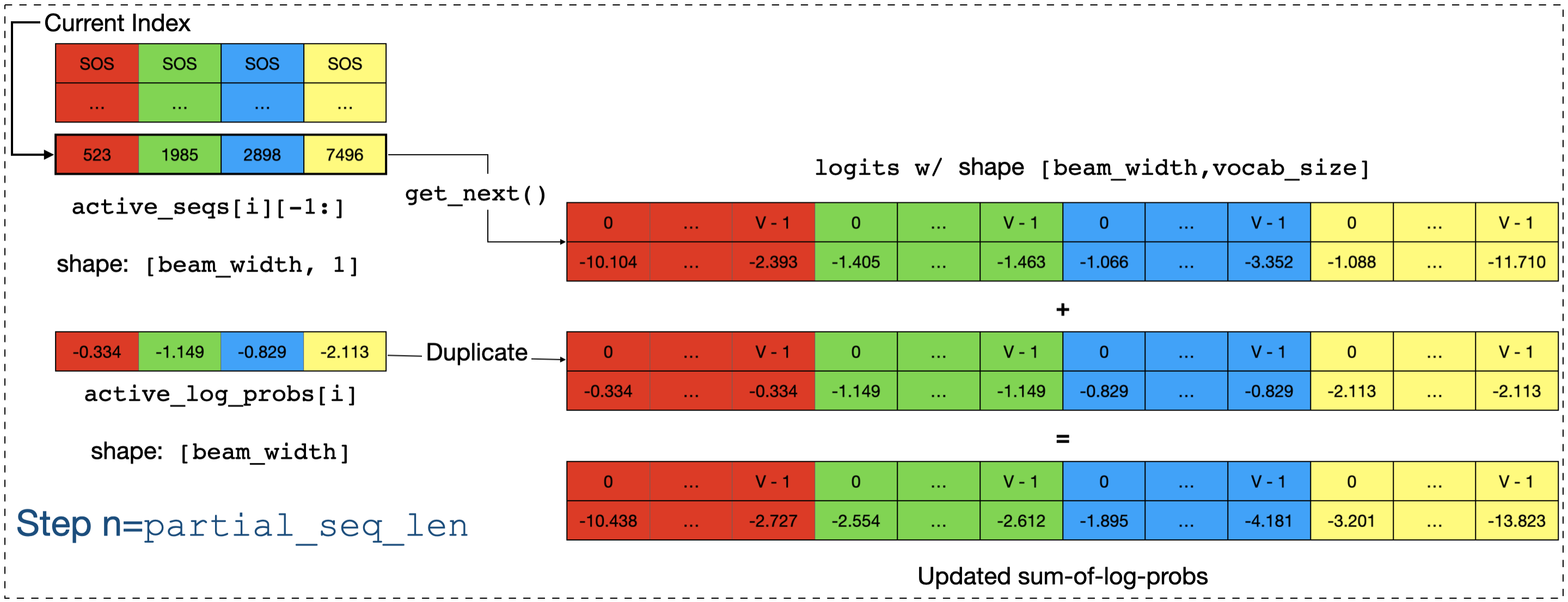
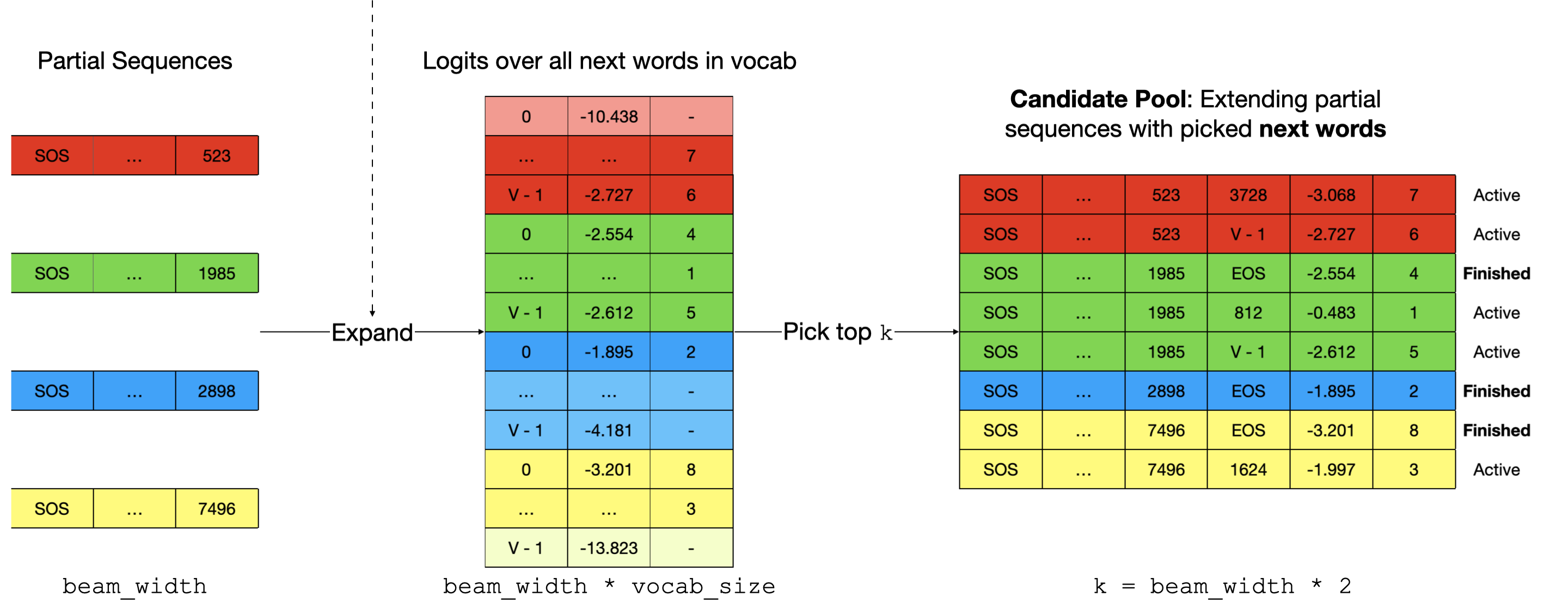
Figure 8: How the "frontiers" of the exploration are expanded and pruned.

We first need to evaluate the likelihood of each word in the vocabulary being the next word of the current set of candidate partial sequences active_seqs[i]. We call the function get_next() that outputs the logits of each potential next word whose index ranges from 0 to vocab_size - 1. The logits will be converted to log-prob and added to the existing sum-of-log-probs active_log_probs[i]. We will reduce the set of candidate partial sequences from beam_width * vocab_size to k = beam_width * 2 by picking the top k scoring candidates (“Candidate Pool” in Figure 7 and 8).

The reason k is beam_width * 2 as opposed to beam_width is that we have to make sure the number of active sequences is still beam_width at the end of each step, and letting k = beam_width * 2 guarantees that we would always end up with at least beam_width active sequences to pick from (convince yourself this is so).

def grow_active_seqs(active_seq, active_log_probs, active_cache, get_next):
  """Grows the search tree of the active sequences by one level, and gathers
  the top-scoring `2 * beam_width` candidates.

  Args:
    active_seq: tensor of shape [batch_size, beam_width, partial_seq_len]
    active_log_probs: tensor of shape [batch_size, beam_width]
    active_cache: nested dict containing tensors of shape [batch_size,
      beam_width, ...]
    get_next: a callable that computes the logits of next words.

  Returns:
    updated_seq: tensor of shape [batch_size, beam_width * 2,
      partial_seq_len + 1]
    updated_log_probs: tensor of shape [batch_size, beam_width * 2]
    updated_active_cache: nested dict containing tensors of shape [batch_size,
      beam_width * 2, ...]
  """
  pass

As shown in the function signature of grow_active_seqs, the input arguments active_seq and active_log_probs maintain the status of active sequences. active_cache keeps track of the status of words that have been generated earlier than the “current word” (for example, the already computed key and value vectors of words that we pay attention to in the Transformer model, or the recurrent state vectors in RNN sequence model), which will be updated as well in this function. get_next is a callback function that computes the logits (equivalently the prob distribution) of next words, and will be executed within grow_active_seqs.

Gather Top Active Sequences

Given the beam_width * 2 candidates in which at least beam_width are active, it would be straightforward to pick & gather top beam_width scoring active parital sequences.

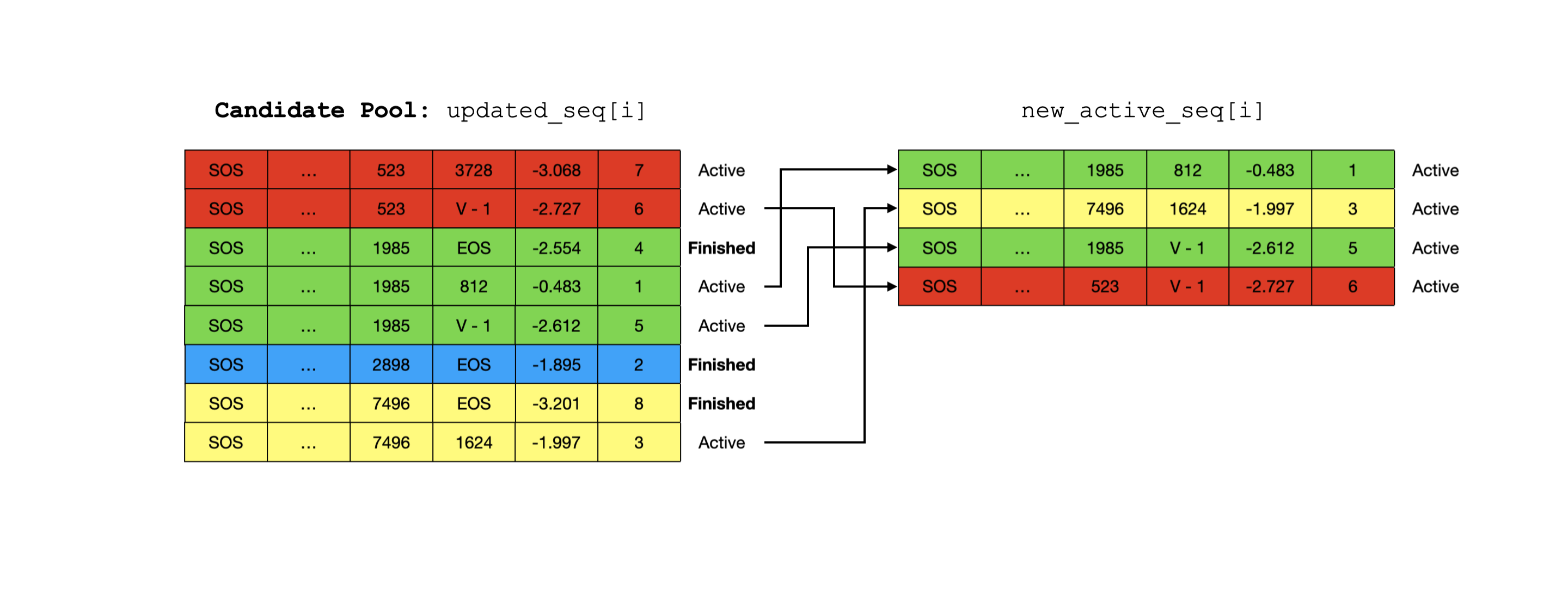
Figure 9: Gather top active sequences. The active sequence with sum-of-log-prob -3.068 was NOT picked because it's not ranked among the top "beam_width".

def gather_top_active_seqs(
    updated_seq, updated_log_probs, updated_active_cache):
  """Gather top scoring active sequences from the candidate pool.
  Args:
    updated_seq: tensor of shape [batch_size, beam_width * 2, 
      partial_seq_len + 1]
    updated_log_probs: tensor of shape [batch_size, beam_width * 2]
    updated_active_cache: nested dict containing tensors of shape [batch_size,
      beam_width * 2, ...]

  Returns:
    new_active_seq: tensor of shape [batch_size, beam_width,
      partial_seq_len + 1]
    new_log_probs: tensor of shape [batch_size, beam_width]
    new_active_cache: nested dict containing tensors of shape [batch_size,
      beam_width, ...]
  """
  pass 

Gather Top Finished Sequences

Unlike the case for active sequences, it will be a little more complicated to update the finished sequences because not only do we need to pick finished sequences from the Candidate Pool, but also cross-check with those that are already finished in previous steps. We need to combine the new and the old and pick the top beam_width scoring finished sequences.

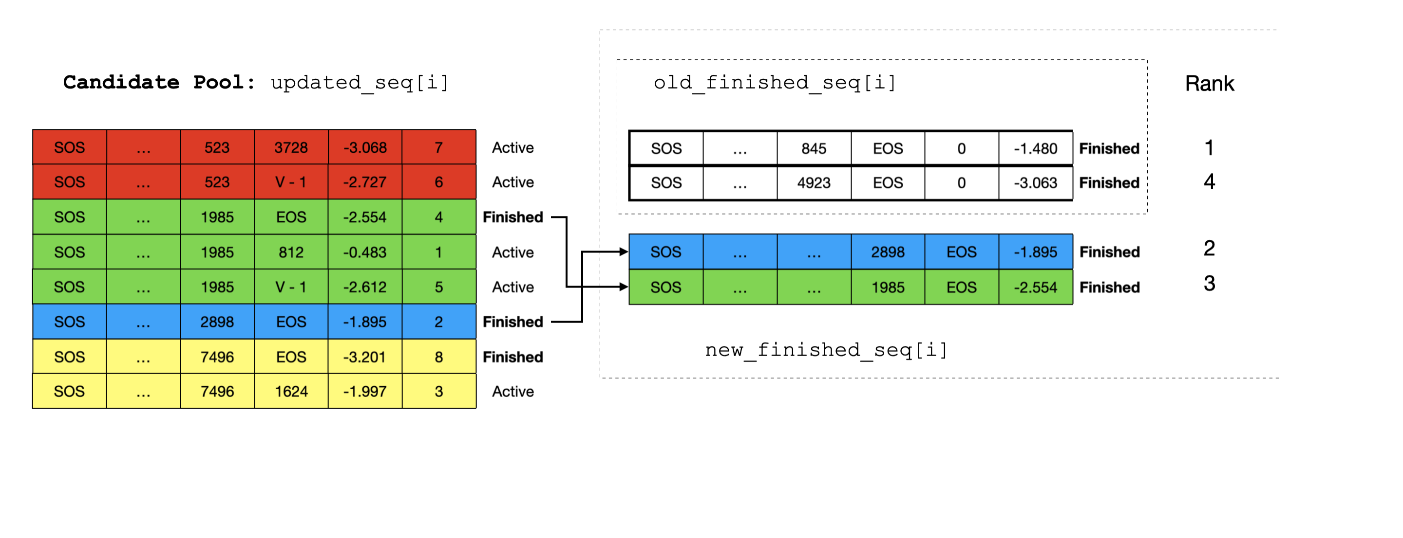
Figure 10: Gather top finished sequences. The sequences finished in previous steps are colored in white. We combine those picked from the Candidate Pool with those that are previously finished, and pick the top scoring ones. Note that the previously finished sequences are shorter and will be zero-padded to match the length of those picked from the Candidate Pool.

def gather_top_finished_seqs(
    updated_seq, updated_log_probs, old_finished_seq, old_finished_score):
  """
  Args:
    updated_seq: tensor of shape [batch_size, beam_width * 2, 
      partial_seq_len + 1]
    updated_log_probs: tensor of shape [batch_size, beam_width * 2]
    old_finished_seq: tensor of shape [batch_size, num_finished, 
      partial_seq_len]
    olf_finished_score: tensor of shape [batch_size, num_finished] 

  Returns:
    new_finished_seq: tensor of shape [batch_size, beam_width, 
      partial_seq_len + 1]
    new_finished_score: tensor of shape [batch_size, beam_width]
  """
  pass

When to Terminate Search

We haven’t talked about when we should stop searching. Typically, we specify a hyperparameter max_seq_len that controls the maximum number of words a sequence can have. We terminate the growth of a sequence when the length reaches max_seq_len.

Is there any other scenario where the searching should be terminated even before max_seq_len is reached? Remember that the sum-of-log-probs of active partial sequencs are always updated by adding a negative value (i.e. log-prob of the “next words”). So if the maximum sum-of-log-prob of active sequences is less than the minimum sum-of-log-prob of finished sequences (over all beams), the active sequences would never overtake finished ones in terms of the sum-of-log-prob scores, and we should stop searching as there will be no newly finished sequences.

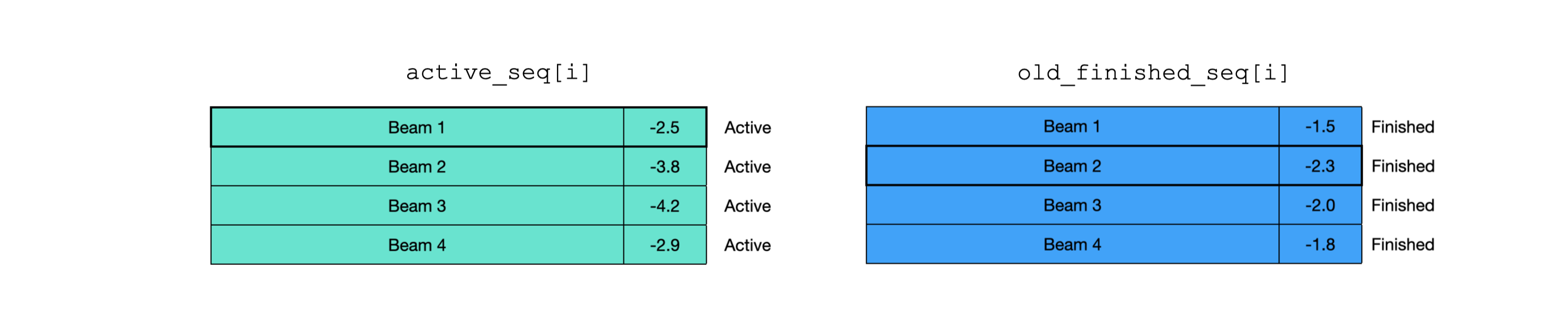
Figure 11: The scenario where we should stop updating the status of active and finished sequences.

Implementation in Python & TensorFlow

A reference implementation is available here. You need to create an instance of BeamSearch where a callable get_next is supplied that computes the logits of next words (check the function signature listed below). Then call the instance method search that returns the finished sequences found by Beam Search. For examples that performs Beam Search using this implementation, refer to Transformer and Seq2Seq.

class BeamSearch(object):
  def __init__(self, 
               get_next, 
               vocab_size,
               batch_size,
               beam_width,
               alpha,
               max_decode_length,
               eos_id):
    pass

  def search(self, initial_ids, initial_cache):
    """Searches for sequences with greatest log-probs.

    Args:
      initial_ids: tensor of shape [batch_size] 
      initial_cache: nested dict containing tensors of shape [batch_size,
        beam_width, ...] 

    Returns:
      finished_seqs: tensor of shape [batch_size, beam_width, seq_len]
      finished_scores: tensor of shape [batch_size, beam_width]
    """
    pass

def get_next(inputs):
  """Compute logits based on input word IDs.
  Args:
    inputs: tensor of shape [batch_size, 1]

  Returns:
    logits: tensor of shape [batch_size, vocab_size]
  """
  decoder_inputs = get_embedding(inputs) #[batch_size, hidden_size]
  logits = compute_logits(decoder_inputs) #[batch_size, vocab_size]
  return logits