From Likelihood Maximization to Loss Minimization

Loss function is an important component for almost all Machine Learning models, especially neural networks. It compares the prediction that comes out of the model with the groundtruth, and determines how dissimilar they are (i.e. how bad the prediction is). For example, a ConvNet-based object detector performs both the classification task and the regression task — it predicts a vector $p_{cls}$ holding the confidence scores corresponding to different object classes, and another vector $p_{loc}$ describing how the anchor boxes should be shifted and scaled so it can tightly bound the object instances. To measure the quality of the predictions, we compute the cross-entropy loss (Sigmoid or Softmax) for classification task, and Huber loss (a variant of squared error loss) for regression task, between the predictions and their respective groundtruths, and we tune the neural network weights to minimize the losses.

You may wonder why cross-entropy loss and squared-error loss are chosen for classification and regression tasks. In this post I’ll try to justify the choices by providing a probabilistic interpretation of different loss functions. To simplify the disscussion, I’ll use the simplest form of each task — logistic regression and linear regression, as our running examples.

Problem Setup

Logistic regression and linear regression are two closely related and well-established techniques in Statistics. They both take as input $n$ observations, each represented as a $d$-dimensional row vector, describing different attributes of a given observation (e.g. height and weight of a person). Also, each observation comes with a label, which is discrete-valued (e.g. 1 or 0) for logistic regression, or continuously valued (e.g. 1.8) for linear regression. Formally, the observations are represented as a $n \times (d + 1)$ matrix $\mathbf{X}$, and the labels are represented as a column vector $\mathbf{y}$, that is

$$\mathbf{X} = \begin{pmatrix} 1 & x_{11} & x_{12} & \cdots & x_{1d} \\ 1 & x_{21} & x_{22} & \cdots & x_{2d} \\ \vdots & \vdots & \ddots & \vdots \\ 1 & x_{n1} & x_{n2} & \cdots & x_{nd} \end{pmatrix} = \begin{pmatrix} \mathbf{x}_{1}^{T} \\ \mathbf{x}_{2}^{T} \\ \vdots \\ \mathbf{x}_{n}^{T} \\ \end{pmatrix} \text{,} \mathbf{y} = \begin{pmatrix} y_{1} \\ y_{2} \\ \vdots \\ y_{n} \end{pmatrix}$$

where $n$ is the number of observations and $d$ is the number of attributes (or features). Note: to accommodate the additional constant $w_{0}$ and to simplify notation (See below), we prefixed the $n \times d$ matrix with a column of ones.

To generate the predictions, we apply a linear transformation on each observation (i.e. $\mathbf{x}_{i}^{T}$, row of $\mathbf{X}$) — a linear combination of attributes plus a constant. Formally, the predicted values are

$$\mathbf{\hat{y}} = \begin{pmatrix} \hat{y}_{1} \\ \hat{y}_{2} \\ \vdots \\ \hat{y}_{n} \end{pmatrix} = \begin{pmatrix} w_{0} + x_{11}w_{1} + x_{12}w_{2} + \cdots + x_{1d}w_{d}\\ w_{0} + x_{21}w_{1} + x_{22}w_{2} + \cdots + x_{2d}w_{d}\\ \vdots \\ w_{0} + x_{n1}w_{1} + x_{n2}w_{2} + \cdots + x_{nd}w_{d} \end{pmatrix} = \mathbf{X} \mathbf{w} = \begin{pmatrix} \mathbf{x}_{1}^{T} \mathbf{w} \\ \mathbf{x}_{2}^{T} \mathbf{w} \\ \vdots \\ \mathbf{x}_{n}^{T} \mathbf{w} \\ \end{pmatrix}$$

where

$$\mathbf{w} = \begin{pmatrix} w_{0} \\ w_{1} \\ \vdots \\ w_{d} \end{pmatrix}$$

For linear regression, we’ll output the prediction $\mathbf{\hat{y}}$ unchanged. However, for logistic regression, we’ll output an indicator vector, which takes the value of 1 if $\hat{\mathbf{y}} \ge 0$, and 0 otherwise.

Model label and observations as random variables

The attributes of the observations $\mathbf{X}$ as well as the labels $\mathbf{y}$ are referred to as training data, and they are fixed once the process of collecting the training data is finished. However, this process itself may involve certain degree of stochasticity — we may end up collecting a different set of values for $\mathbf{X}$ if we were to repeat the collecting process; and even if we happen to get the same set of values for $\mathbf{X}$ as previously collected, the values for the labels $\mathbf{y}$ may still be different. As a result, we usually model the labels and observations as random variables, so $\mathbf{y}$ and $\mathbf{X}$ are just concrete values that the random variables can take on.

Formally, given that the training set contains $n$ observations with $d$ attributes, we use the random variable $Y_{i}$ ($i= 1, \cdots, n$) to denote the label for the $i$th observation, and random variables $X_{i1}, X_{i2}, \cdots, X_{id}$ to denote its attributes. So $Y_{i}$ takes on the value of each component of $\mathbf{y}$, and $X_{i1}, X_{i2}, \cdots, X_{id}$ take on each row of $\mathbf{X}$.

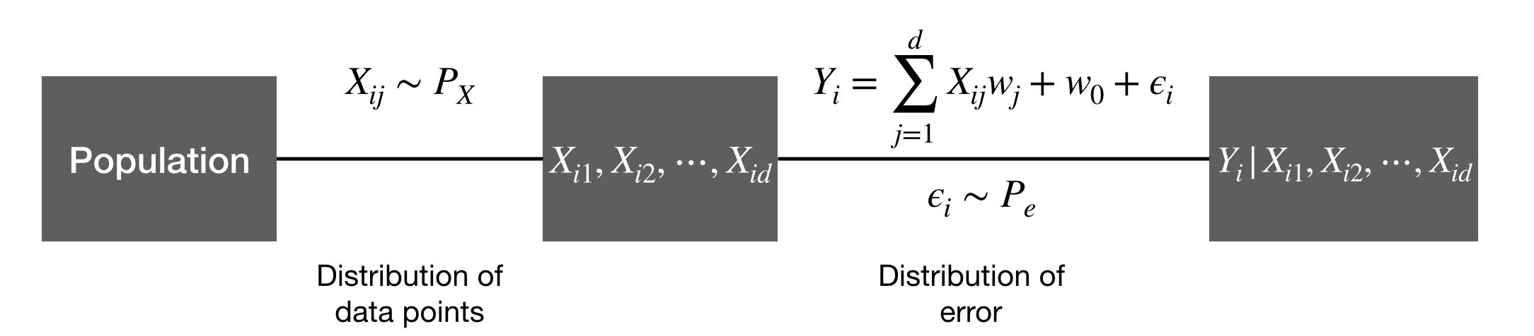
Sample a set of data points with observations, and then sample the corresponding labels.

Note that the stochasticity associated with the random variables $X_{i1}, X_{i2}, \cdots, X_{id}$ is determined by the distribution of samples in a population — we first sample (randomly) a set of data points according to the distribution, then record their attributes; However, the stochasticity associated with $Y_{i}$ is determined by both the distribution of samples (to determine $Y_{i}$ we first need to sample a data point $i$), and the inevitable error assosicated the labelling the data point $i$ (e.g. the measured height may always be slightly different from the true height of an individual). For our discussion, we’ll treat the $X_{ij}$ as fixed, and only discuss $P(Y_{i} \vert X_{i1}, X_{i2}, \cdots, X_{id})$ — the probability of $Y_{i}$ conditioned on $X_{i1}, X_{i2}, \cdots, X_{id}$, whose randomness is attributed to the labelling error.

The error distribution

To account for the labelling error, we’ll add an error term $\epsilon_{i}$ to the linear transformation of $X_{i1}, X_{i2}, \cdots, X_{id}$, and denote the result as

$$Y_{i}^{*} = \sum_{j=1}^{d} X_{ij} w_{j} + w_{0} + \epsilon_{i} \tag{1}$$

As discussed previously, for linear regression the label (or the predicted label) $Y_{i}$ is just the linear combination (plus the error), so

$$Y_{i} = Y_{i}^{*} \tag{2}$$

,while for logistic regression, we add a binarization step:

$$Y_{i} = \begin{cases} 1, \text{ if } Y_{i}^{*} \ge 0 \\ 0, \text{ if } Y_{i}^{*} \lt 0 \tag{3} \end{cases}$$

As for the error term’s distribution, we assume it follows a zero-mean normal distribution,

$$\epsilon_{i} \sim \mathcal{N}(0, \sigma^{2})$$

for linear regression, and a logistic distribution with location being 0 and scale being 1 for logistic regression.

$$\epsilon_{i} \sim \text{Logistic}(0, 1)$$

We assume that each data point is labelled independently, so $\epsilon_{i}$ and hence $Y_{i}$ should be i.i.d. (independently and identically distributed).

Maximizing the Likelihood

Now we are ready to derive the probability of $Y_{i}$ conditioned on $X_{i1}, X_{i2}, \cdots, X_{id}$ analytically, i.e, $P(Y_{i} = y_{i} \vert X_{i1} = x_{i1}, X_{i2}=x_{i2}, \cdots, X_{id}=x_{id}; \mathbf{w})$. We’ll find the $\mathbf{w}$ that maximizes the logarithm of probability, which is equivalent to maximizing the probability itself.

Linear regression

Given equations (1), (2), and $\epsilon_{i} \sim \mathcal{N}(0, \sigma^{2})$, it follows that $Y_{i}$ is a continuous random variable, and $Y_{i} \vert X_{i1}, X_{i2}, \cdots, X_{id} \sim \mathcal{N}(\mathbf{x}_{i}^{T} \mathbf{w}, \sigma^{2})$. Maximizing the log-likelihood, we have

$$\begin{align} &\arg\max_{\mathbf{w}} L(\mathbf{w}) \\ = &\arg\max_{\mathbf{w}} \log P(Y_{i} = y_{i} \vert X_{i1} = x_{i1}, X_{i2}=x_{i2}, \cdots, X_{id}=x_{id}; \mathbf{w}) \\ = &\arg\max_{\mathbf{w}} \log \frac{1}{\sqrt{2\pi} \sigma} e^{-\frac{(y_{i} - \mathbf{x}_{i}^{T} \mathbf{w} )^2}{2\sigma^{2}}} \\ = & \arg\max_{\mathbf{w}} \log e^{-\frac{(y_{i} - \mathbf{x}_{i}^{T} \mathbf{w} )^2}{2\sigma^{2}}} \\ = & \arg\min_{\mathbf{w}} (y_{i} - \mathbf{x}_{i}^{T} \mathbf{w} )^2 \end{align}$$

We have just proved that maximizing the likelihood is equivalent to minimizing the squared error.

Logistic regression

Given equations (1) and (3), it follows that $Y_{i}$ is a discrete random variable that takes on the value of 0 or 1, and $Y_{i} = 1$ iff $Y_{i}^{*} \ge 0$. We have

$$\begin{align} & P(Y_{i} = 1 \vert X_{i\cdot} = x_{i\cdot}; \mathbf{w}) \\ = & P(Y_{i}^{*} \ge 0 \vert X_{i\cdot} = x_{i\cdot}; \mathbf{w}) \\ = & P(\mathbf{x}_{i}^{T} \mathbf{w} + \epsilon_{i} \ge 0 \vert X_{i\cdot} = x_{i\cdot}; \mathbf{w} ) \\ = & P(\epsilon_{i} \ge - \mathbf{x}_{i}^{T} \mathbf{w} \vert X_{i\cdot} = x_{i\cdot}; \mathbf{w} ) \\ = & P(\epsilon_{i} \le \mathbf{x}_{i}^{T} \mathbf{w} \vert X_{i\cdot} = x_{i\cdot}; \mathbf{w}) \\ = & \frac{1}{1 + e^{-\mathbf{x}_{i}^{T} \mathbf{w}}} \end{align}$$

where $X_{i\cdot} = x_{i\cdot}$ denotes $X_{i1} = x_{i1}, X_{i2}=x_{i2}, \cdots, X_{id}=x_{id}$.

The last two steps follows from the fact that $\epsilon_{i} \sim \text{Logistic}(0, 1)$, and its cumulative distribution function is just the logistic function, i.e. $P(\epsilon_{i} \le x) = \frac{1}{1 + e^{-x}}$, and $P(\epsilon_{i} \gt -x) = 1 - P(\epsilon_{i} \le -x) = 1 - \frac{1}{1 + e^{x}} = \frac{1}{1 + e^{-x}} = P(\epsilon_{i} \le x)$

It follows that $Y_{i} \vert X_{i1}, X_{i2}, \cdots, X_{id} \sim \text{Bernoulli}(\frac{1}{1 + e^{-\mathbf{x_{i}}^{T} \mathbf{w}}})$.

Maximizing the log-likelihood, we have

$$\begin{align} &\arg\max_{\mathbf{w}} L(\mathbf{w})\\ = & \arg\max_{\mathbf{w}} \log P(Y_{i} = y_{i} \vert X_{i1}, X_{i2}, \cdots, X_{id}; \mathbf{w}) \\ = & \arg\max_{\mathbf{w}} \log P(Y_{i} = 1 \vert X_{i1}, X_{i2}, \cdots, X_{id}; \mathbf{w})^{y_{i}} P(Y_{i} = 0 \vert X_{i1}, X_{i2}, \cdots, X_{id}; \mathbf{w})^{1 - y_{i}} \\ = & \arg\max_{\mathbf{w}} y_{i} \log \left( \frac{1}{1 + e^{-\mathbf{x}_{i}^{T} \mathbf{w}}} \right) + (1 - y_{i}) \log \left( 1 - \frac{1}{1 + e^{-\mathbf{x}_{i}^{T} \mathbf{w}}} \right) \\ = & \arg\min_{\mathbf{w}} \left(-y_{i} \log \left( \frac{1}{1 + e^{-\mathbf{x}_{i}^{T} \mathbf{w}}} \right) - (1 - y_{i}) \log \left( 1 - \frac{1}{1 + e^{-\mathbf{x}_{i}^{T} \mathbf{w}}} \right) \right) \end{align}$$

Again, we have proved that maximizing the likelihood is equivalent to minimizing the cross-entropy, which is defined between the target distribution (Bernoulli) $(y_{i}, 1 - y_{i})$ and predicted distribution $(\frac{1}{1 + e^{-\mathbf{x}_{i}^{T} \mathbf{w}}}, 1 - \frac{1}{1 + e^{-\mathbf{x}_{i}^{T} \mathbf{w}}})$.

Miminize the loss

At this point, it’ll be trivial to derive the update algorithm to optimize the losses.

Linear regression

Let the loss function $J(\mathbf{w}) = \frac{1}{2} (y_{i} - \mathbf{x}_{i}^{T} \mathbf{w} )^2$. Using chain rule, we have

$$\frac{\partial}{\partial w_{j}} J(\mathbf{w}) = (y_{i} - \mathbf{x}_{i}^{T} \mathbf{w} ) (-x_{ij}) = (\mathbf{x}_{i}^{T} \mathbf{w} - y_{i}) x_{ij}$$

Logistic regression

Let $h(\mathbf{x_{i}^{T}}) = \frac{1}{1 + e^{-\mathbf{x}^{T} \mathbf{w}}}$ and the loss function $J(\mathbf{w}) = -y_{i} \log h(\mathbf{x_{i}^{T}}) - (1 - y_{i}) \log (1 - h(\mathbf{x_{i}^{T}}))$. Using chain rule, we have

$$\begin{align} & \frac{\partial}{\partial w_{j}} J(\mathbf{w}) \\ = & \frac{\partial}{\partial w_{j}} \left(-y_{i} \log h(\mathbf{x_{i}^{T}}) - (1 - y_{i}) \log (1 - h(\mathbf{x_{i}^{T}})) \right) \\ = & -\frac{y_{i}}{h(\mathbf{x_{i}^{T}})} \frac{\partial}{\partial w_{j}} h(\mathbf{x_{i}^{T}}) + \frac{1 - y_{i}}{ 1 - h(\mathbf{x_{i}^{T}})} \frac{\partial}{\partial w_{j}} h(\mathbf{x_{i}^{T}}) \\ = & \left( \frac{1 - y_{i}}{1 - h(\mathbf{x_{i}^{T}}) } - \frac{y_{i}}{ h(\mathbf{x_{i}^{T}}) } \right) \frac{\partial}{\partial w_{j}} h(\mathbf{x_{i}^{T}}) \\ = & \left( \frac{1 - y_{i}}{1 - h(\mathbf{x_{i}^{T}}) } - \frac{y_{i}}{ h(\mathbf{x_{i}^{T}}) } \right) (1 - h(\mathbf{x_{i}^{T}})) h(\mathbf{x_{i}^{T}}) x_{ij} \\ = & (h(\mathbf{x_{i}^{T}}) - y_{i}) x_{ij} \end{align}$$

It’s a little surprising that we end up with almost identical update algorithm for both logistic regression and linear regression. In both algorithms, the magnitude of the update depends on the error $h(\mathbf{x_{i}^{T}}) - y_{i}$ or $\mathbf{x}_{i}^{T} \mathbf{w} - y_{i}$, which means if we made a big error in the prediction, we should accordingly make a large stride to update the corredponding weight.

Summary

In this post, we provided a probabilistic interpretation for the principle of loss minimization for linear regression and logistic regression. We discussed the sources of randomness for both labels and inputs, and modeled the labels as random variables conditioned on the observed inputs. We gave assumptions on the probability distributions of the errors, and finally showed that maximizing the likelihood of the labels is equivalent to minimizing the squared error loss or cross entropy loss.