SVD Explained

In the previous post we talked about Principlal Component Analysis, a popular statistical technique for dimensionality reduction and feature decorrelation. Another common use case is matrix decomposition, where a matrix is factorized into a product of matrices (Eigendecomposition).

A limitation of Eigendecomposition is that it only works on square matrices. Singular Value Decomposition (SVD) is a generalization of Eigendecomposition, which works on any rectangle-shaped matrix. It has been widely used in Machine Learning applications such as Latent Semantic Analysis (LSA), where a document-word matrix is decomposed and re-represented while keeping the pattern in the original matrix, and image compression, where a matrix holding the pixel intensities is decomposed and re-represented as the product of three much smaller matrices, from which the original image can be reconstructed.

In this post, I’ll explain mathematically why a Singular Value Decomposition always exists for any rectangle-shaped matrix, and how to find it. It is assumed that you have some basic grasp of Linear Algebra (I recommend you to read the post on PCA).

The Math

Let $A$ be any $m \times n$ real-valued matrix where $m \le n$. It can be shown that the $m \times m$ matrix $AA^{T}$ is

1. symmetric
2. positive semidefinite

Let $\lambda_{1}, \lambda_{2}, \cdots, \lambda_{m}$ be the $m$ eigenvalues of $AA^{T}$, and $u_{1}, u_{2}, \cdots, u_{m}$ be the eigenvectors (column vectors of shape $m \times 1$) corresponding to $\lambda_{1}, \lambda_{2}, \cdots, \lambda_{m}$, respectively. It follows that

$$\begin{align} AA^{T}u_{1} &= \lambda_{1} u_{1} \\ AA^{T}u_{2} &= \lambda_{2} u_{2} \\ &\cdots \\ AA^{T}u_{m} & = \lambda_{m} u_{m} \\ \end{align}$$

and

• The eigenvalues are non-negative: $\lambda_{1} \ge 0, \lambda_{2} \ge 0, \cdots, \lambda_{m} \ge 0$.
• The eigenvectors (corresponding to different eigenvalues) are pairwise orthogonal: $u_{i}^{T}u_{j} = 0$ for $i \ne j$ and $i, j = 1, \cdots, m$.

We’ll further assume that $u_{1}, u_{2}, \cdots, u_{m}$ are unit vectors:

$u_{i}^{T}u_{i} = 1$ for $i = 1, \cdots, m$.

 

Let’s define another $m$ column vectors $v_{i}$ (of shape $n \times 1$):

$v_{i} = \frac{1}{\sqrt{\lambda_{i}}} A^{T}u_{i}$ for $i = 1, \cdots, m$

We can show that

$$\begin{align} A^{T}Av_{i} & = A^{T}A \frac{1}{\sqrt{\lambda_{i}}} A^{T} u_{i} = \frac{1}{\sqrt{\lambda_{i}}} A^{T} A A^{T} u_{i} \\ &= \frac{1}{\sqrt{\lambda_{i}}} A^{T} \lambda_{i} u_{i} = \sqrt{\lambda_{i}} A^{T} u_{i} = \sqrt{\lambda_{i}} \sqrt{\lambda_{i}} v_{i} = \lambda_{i} v_{i} \end{align}$$

In other words, $\lambda_{i}$’s are also eigenvalues of the $n \times n$ of matrix $A^{T}A$, and $v_{i}$’s are the eigenvectors corresponding to $\lambda_{i}$, for $i = 1, \cdots, m$

and $v_{i}$’s are unit vectors too:

$$\begin{align} v_{i}^{T}v_{i} & = \frac{1}{\sqrt{\lambda_{i}}} u_{i}^{T} A \cdot \frac{1}{\sqrt{\lambda_{i}}} A^{T}u_{i} \\ & = \frac{1}{\lambda_{i}} u_{i}^{T} A A^{T} u_{i} = \frac{1}{\lambda_{i}} u_{i}^{T} \lambda_{i} u_{i} = u_{i}^{T} u_{i} = 1 \end{align}$$

Note that $A^{T} A$ is a $n \times n$ matrix and $n \ge m$, so it might have additional eigenvalues $\lambda_{m + 1}, \lambda_{m + 2}, \cdots, \lambda_{n}$, with the corresponding eigenvectors $v_{m+1}, v_{m+2}, \cdots, v_{n}$, respectively. Because the eigenvectors $v_{1}, v_{2}, \cdots, v_{m}, v_{m+1}, \cdots, v_{n}$ correspond to different eigenvalues, they must be pairwise orthogonal:

$v_{i}^{T}v_{j} = 0$ for $i \ne j$ and $i, j = 1, \cdots, n$

 

 

Finally, let’s put together the two groups of eigenvectors into a $m \times m$ matrix $U$ and a $n \times n$ matrix $V$, where

$$U = \begin{bmatrix}u_{1}^{T}\\u_{2}^{T} \\ \vdots \\ u_{m}^{T}\end{bmatrix}$$

and

$$V = \begin{bmatrix} v_{1} & v_{2} & \cdots & v_{m} & v_{m+1} & \cdots& v_{n} \end{bmatrix}$$

Note that both $U$ and $V$ are inversible because their rows/columns are pairwise orthogonal (hence linearly independent).

Let’s compute the product of three matrices $U$, $A$ and $V$:

$$\begin{align} U A V & = \begin{bmatrix}u_{1}^{T}\\u_{2}^{T} \\ \vdots \\ u_{m}^{T}\end{bmatrix} \cdot A \cdot \begin{bmatrix} v_{1} & v_{2} & \cdots & v_{m} & v_{m+1} & \cdots& v_{n} \end{bmatrix} \\ & = \begin{bmatrix} u_{1}^{T}A \\ u_{2}^{T}A \\ \vdots \\ u_{m}^{T}A\end{bmatrix} \cdot \begin{bmatrix}v_{1} & v_{2} & \cdots & v_{m} & v_{m + 1} & \cdots & v_{n} \end{bmatrix} \\ & = \begin{bmatrix} u_{1}^{T}Av_{1} & u_{1}^{T}Av_{2} & \cdots & u_{1}^{T}Av_{m} & u_{1}^{T}Av_{m+1} & \cdots & u_{1}^{T}Av_{n} \\ u_{2}^{T}Av_{1} & u_{2}^{T}Av_{2} & \cdots & u_{2}^{T}Av_{m} & u_{2}^{T}Av_{m+1} & \cdots & u_{2}^{T}Av_{n} \\ \vdots & \vdots & & \vdots & \vdots & & \vdots \\ u_{m}^{T}Av_{1} & u_{m}^{T}Av_{2} & \cdots & u_{m}^{T}Av_{m} & u_{m}^{T}Av_{m+1} & \cdots & u_{m}^{T}Av_{n} \end{bmatrix} \end{align}$$

Remember that we defined $v_{i} = \frac{1}{\sqrt{\lambda_{i}}} A^{T}u_{i}$, where $i = 1, \cdots, m$.

It follows that $u_{i}^{T} A = \sqrt{\lambda_{i}} v_{i}^{T}$ for $i = 1, \cdots, m$

Therefore for $i = 1, \cdots, m$ and $j = 1, \cdots, n$,

$$u_{i}^{T} A v_{j} = \sqrt{\lambda_{i}} v_{i}^{T} v_{j} = \begin{cases} \sqrt{\lambda_{i}}, & 1 \le i = j \le m \\ 0, & i \ne j \end{cases}$$

So

$$UAV = \begin{bmatrix} \sqrt{\lambda_{1}} & & \cdots & & & \cdots & \\ & \sqrt{\lambda_{2}} & \cdots & & & \cdots & \\ \vdots & \vdots & & \vdots & \vdots & & \vdots \\ & & \cdots & \sqrt{\lambda_{m}} & & \cdots & \end{bmatrix} = \Sigma$$

and the SVD of A is $A = U^{-1} \Sigma V^{-1}$

 

 

Recap: the following are the steps to carry out SVD on any rectangle-shaped matrix $A$ of shape $m \times n$ ($m \le n$)

1. Compute $A A^{T}$ and find its eigenvalues $\lambda_{i}$ and eigenvectors $u_{i}$ for $i = 1, \cdots, m$.
2. Build $m \times m$ matrix $U = \begin{bmatrix}u_{1}^{T}\\u_{2}^{T} \\ \vdots \\ u_{m}^{T}\end{bmatrix}$
3. Build $n \times n$ matrix $V = \begin{bmatrix} v_{1} & v_{2} & \cdots & v_{m} & v_{m+1} & \cdots& v_{n} \end{bmatrix}$, where $v_{i} = \frac{1}{\sqrt{\lambda_{i}}} A^{T}u_{i}$ for $i = 1, \cdots, m$, and $v_{m + 1}, \cdots, v_{n}$ are eigenvectors of $A^{T}A$ corresponding to eigenvalues $\lambda_{m + 1}, \cdots, \lambda_{n}$ that are not eigenvalues of $AA^{T}$.

4. Build matrix $\begin{bmatrix} \sqrt{\lambda_{1}} & & \cdots & & & \cdots & \\ & \sqrt{\lambda_{2}} & \cdots & & & \cdots & \\ \vdots & \vdots & & \vdots & \vdots & & \vdots \\ & & \cdots & \sqrt{\lambda_{m}} & & \cdots & \end{bmatrix}$ of shape $n \times m$

5. Compute $A_{SVD} = U^{-1} \Sigma V^{-1}$

Example

Toy example

First let’s create a small matrix that is easy to test out the theory:

import numpy as np

h = 4
w = 5 # w must be >= h 

A = np.random.randint(0, 255, size=(h, w)).astype('float32')

Find the eigenvalues and eigenvectors of A.dot(A.T) and A.T.dot(A), respectively:

eigval1, eigvec1 = np.linalg.eig(A.dot(A.T))
eigval2, eigvec2 = np.linalg.eig(A.T.dot(A))

Build the matrix U and V:

U = eigvec1.T

# Note: we use `thres` to determine which eigenvalues of `A.T.dot(A)` 
# are NOT eigenvalues of `A.dot(A.T)`
thres = 1e-6
indices = [i for i in range(w) if 
    np.all(np.abs(eigval2[i] - eigval1)) >= thres]

V = np.hstack([A.T.dot(eigvec1) / np.sqrt(eigval1), 
               eigvec2[:, indices].reshape(w, -1)])

Build the matrix Sigma:

Sigma = np.hstack([np.diag(np.sqrt(eigval1)), np.zeros((h, w - h))])

Finaly compute A_SVD (Note U and V are orthonormal matrices so their inverses are identical to their transposed forms):

A_SVD = U.T.dot(Sigma).dot(V.T)

You can see that the reconstructed matrix is identical to the original (up to the error in numerical precision):

print(A)
array([[199., 227., 237., 107., 120.],
       [254., 116., 184., 220., 171.],
       [212., 150.,  85., 195.,  83.],
       [ 24.,  51., 178., 205., 135.]], dtype=float32)

print(np.round(A_SVD))
array([[199., 227., 237., 107., 120.],
       [254., 116., 184., 220., 171.],
       [212., 150.,  85., 195.,  83.],
       [ 24.,  51., 178., 205., 135.]])

Image compression

There is much neater way to carry out SVD than the above precedure. You can use the built-in function of NumPy in one line of code:

u, s, vh = np.linalg.svd(A)

The matrices u and vh are like U.T and V.T as the above example, and s is a 1-D array holding the $\lambda_{i}$’s (a.k.a. Singular Values, hence the name of SVD), and they are by default sorted in descending order. Usually we’d re-represent the original matrix by keeping only the largest Singular Values, and truncate u and vh accordingly. This is known as Truncated SVD.

Code:

import numpy as np
from PIL import Image

def truncated_svd_3_channel_compression(img, t):
  """`img` is 3-D array of shape [height, width, channels]
  `t` is the number of singular values to keep
  """
  u0, s0, vh0 = np.linalg.svd(img[:, :, 0])
  u1, s1, vh1 = np.linalg.svd(img[:, :, 1])
  u2, s2, vh2 = np.linalg.svd(img[:, :, 2])

  r = u0[:, :t].dot(np.diag(s0[:t])).dot(vh0[:t, :])
  g = u1[:, :t].dot(np.diag(s1[:t])).dot(vh1[:t, :])
  b = u2[:, :t].dot(np.diag(s2[:t])).dot(vh2[:t, :])

  return np.stack([r, g, b], axis=2).astype('uint8')


img = np.array(Image.open('img.jpg'))

n10 = truncated_svd_3_channel_compression(img, 10)

Below are the images reconstructed using different number of SV’s as well as the original image. The total number of SV’s is 450 (height of image).

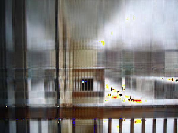
Top 10 (L) and 20 (R) Singular Values

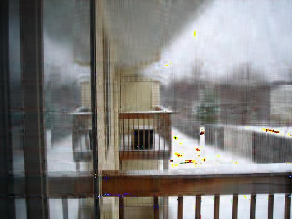
Top 30 (L) and 40 (R) Singular Values

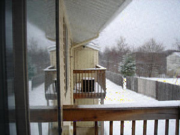
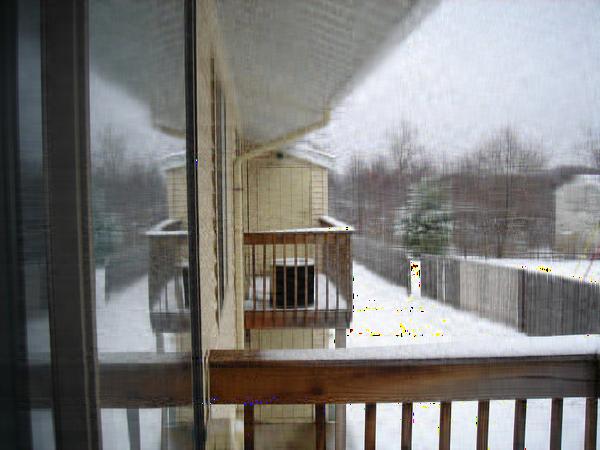
Top 50 (L) Singular Values and orignal image (R)

We can see that as we increase the number of singular values, the reconstructed image gets less blurry and contain less “outlier” pixels, and the one reconstructed from only 50 singular values offers great approximation to the orignal image.